Prepare the HMDB51 Datasetfile_download

hmdb51.py

file_download

Download Python source code: hmdb51.py

file_download

Download Jupyter notebook: hmdb51.ipynb

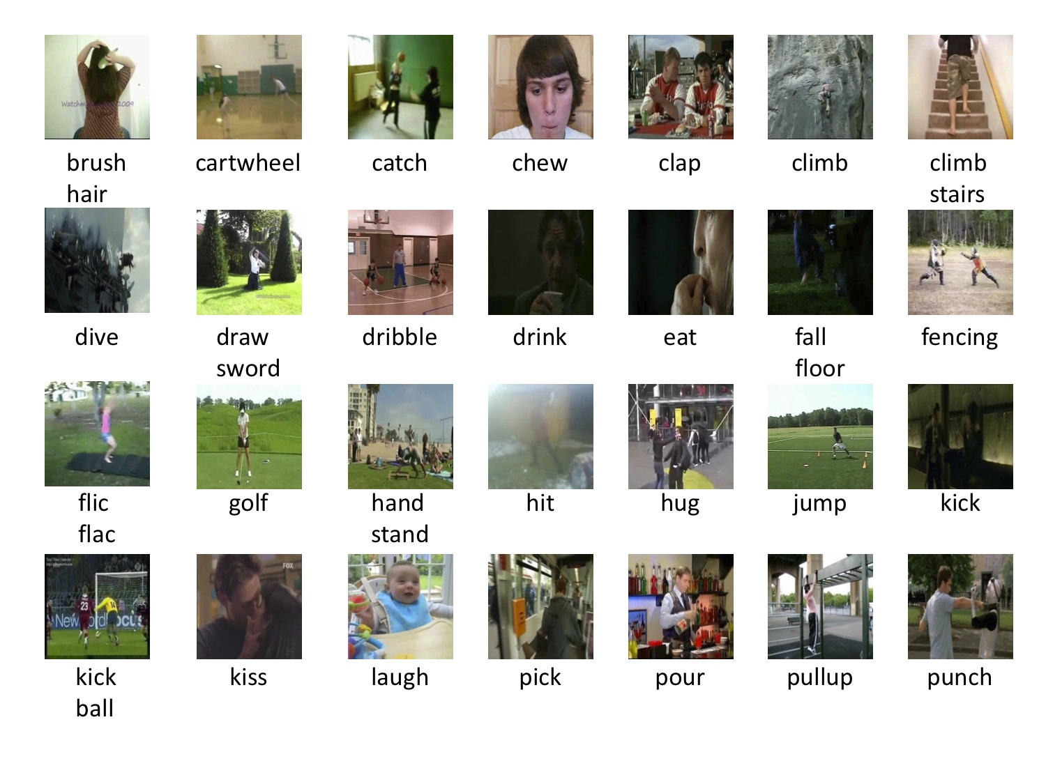
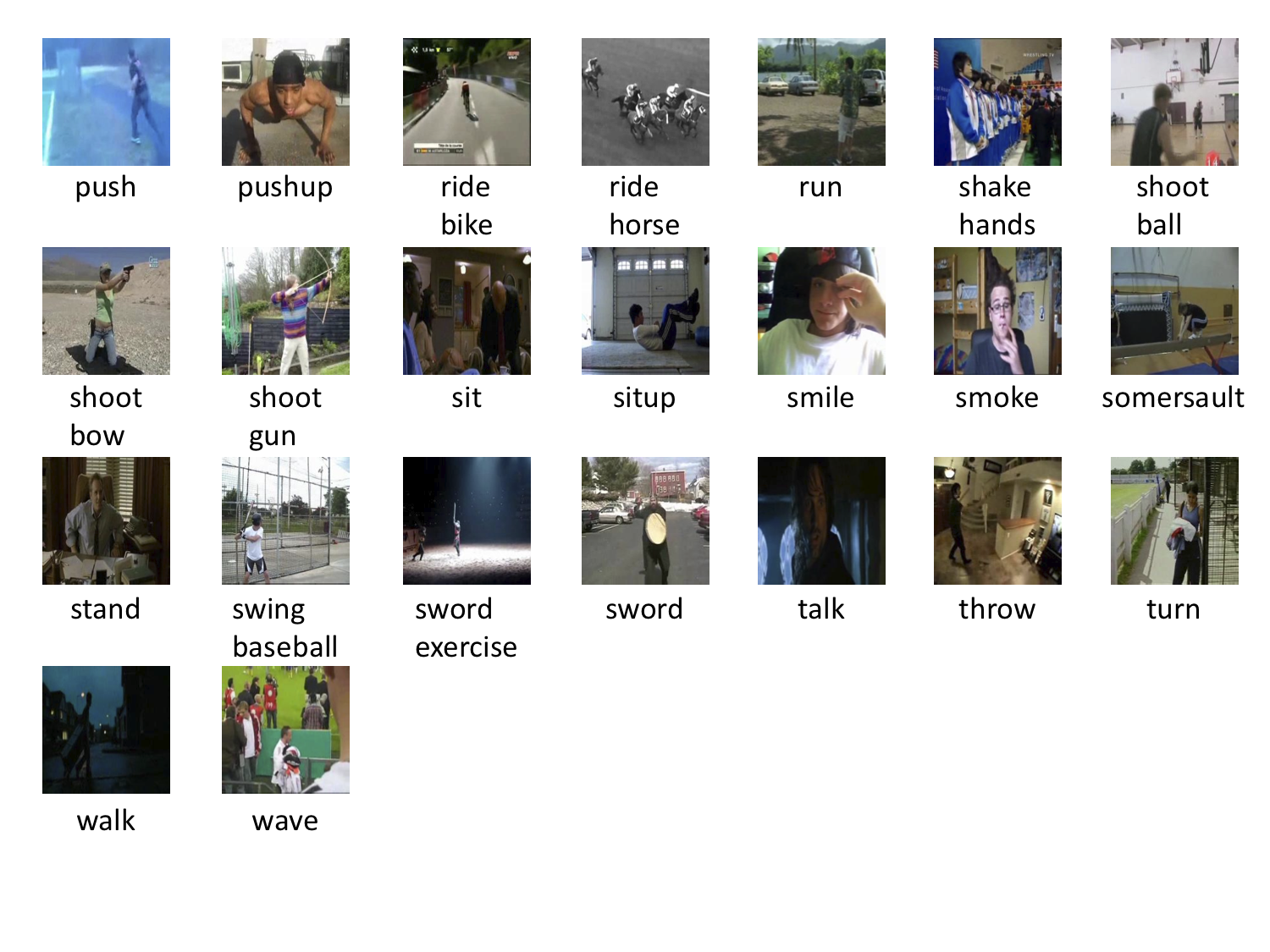
HMDB51 is an action recognition dataset, collected from various sources, mostly from movies, and a small proportion from public databases such as the Prelinger archive, YouTube and Google videos. The dataset contains 6,766 clips divided into 51 action categories, each containing a minimum of 100 clips. This tutorial will go through the steps of preparing this dataset for GluonCV.

Setup

We need the following two files from HMDB51: the dataset and the official train/test split.

Filename	Size
hmdb51_org.rar	2.1 GB
test_train_splits.rar	200 KB

The easiest way to download and unpack these files is to download helper script and run the following command:

python hmdb51.py

This script will help you download the dataset, unpack the data from compressed files, decode the videos to frames, and generate the training files for you. All the files will be stored at ~/.mxnet/datasets/hmdb51 by default. If you want to use more workers to speed up, please specify --num-worker to a larger number.

Note

You need at least 60 GB disk space to download and extract the dataset. SSD (Solid-state disks) is preferred over HDD because of faster speed.

You may need to install unrar by sudo apt install unrar.

You may need to install rarfile, Cython, mmcv by pip install rarfile Cython mmcv.

The data preparation process may take a while. The total time to prepare the dataset depends on your Internet speed and disk performance. For example, it takes about 30min on an AWS EC2 instance with EBS.

Read with GluonCV

The prepared dataset can be loaded with utility class gluoncv.data.HMDB51 directly. In this tutorial, we provide three examples to read data from the dataset, (1) load one frame per video; (2) load one clip per video, the clip contains five consecutive frames; (3) load three clips evenly per video, each clip contains 12 frames.

We first show an example that randomly reads 25 videos each time, randomly selects one frame per video and performs center cropping.

from gluoncv.data import HMDB51
from mxnet.gluon.data import DataLoader
from mxnet.gluon.data.vision import transforms
from gluoncv.data.transforms import video

transform_train = transforms.Compose([
    video.VideoCenterCrop(size=224),
    video.VideoToTensor()
])

# Default location of the data is stored on ~/.mxnet/datasets/hmdb51.
# You need to specify ``setting`` and ``root`` for HMDB51 if you decoded the video frames into a different folder.
train_dataset = HMDB51(train=True, transform=transform_train)
train_data = DataLoader(train_dataset, batch_size=25, shuffle=True)

We can see the shape of our loaded data as below. extra indicates if we select multiple crops or multiple segments from a video. Here, we only pick one frame per video, so the extra dimension is 1.

for x, y in train_data:
    print('Video frame size (batch, extra, channel, height, width):', x.shape)
    print('Video label:', y.shape)
    break

Out:

Video frame size (batch, extra, channel, height, width): (25, 1, 3, 224, 224)
Video label: (25,)

Let’s plot several training samples. index 0 is image, 1 is label

from gluoncv.utils import viz
viz.plot_image(train_dataset[500][0].squeeze().transpose((1,2,0))*255.0)   # dive
viz.plot_image(train_dataset[2500][0].squeeze().transpose((1,2,0))*255.0)  # shoot_bow

• 
• 

Here is the second example that randomly reads 25 videos each time, randomly selects one clip per video and performs center cropping. A clip can contain N consecutive frames, e.g., N=5.

train_dataset = HMDB51(train=True, new_length=5, transform=transform_train)
train_data = DataLoader(train_dataset, batch_size=25, shuffle=True)

We can see the shape of our loaded data as below. Now we have another depth dimension which indicates how many frames in each clip (a.k.a, the temporal dimension).

for x, y in train_data:
    print('Video frame size (batch, extra, channel, depth, height, width):', x.shape)
    print('Video label:', y.shape)
    break

Out:

Video frame size (batch, extra, channel, depth, height, width): (25, 1, 3, 5, 224, 224)
Video label: (25,)

Let’s plot one training sample with 5 consecutive video frames. index 0 is image, 1 is label

from matplotlib import pyplot as plt
# subplot 1 for video frame 1
fig = plt.figure()
fig.add_subplot(1,5,1)
frame1 = train_dataset[500][0][0,:,0,:,:].transpose((1,2,0)).asnumpy()*255.0
plt.imshow(frame1.astype('uint8'))
# subplot 2 for video frame 2
fig.add_subplot(1,5,2)
frame2 = train_dataset[500][0][0,:,1,:,:].transpose((1,2,0)).asnumpy()*255.0
plt.imshow(frame2.astype('uint8'))
# subplot 3 for video frame 3
fig.add_subplot(1,5,3)
frame3 = train_dataset[500][0][0,:,2,:,:].transpose((1,2,0)).asnumpy()*255.0
plt.imshow(frame3.astype('uint8'))
# subplot 4 for video frame 4
fig.add_subplot(1,5,4)
frame4 = train_dataset[500][0][0,:,3,:,:].transpose((1,2,0)).asnumpy()*255.0
plt.imshow(frame4.astype('uint8'))
# subplot 5 for video frame 5
fig.add_subplot(1,5,5)
frame5 = train_dataset[500][0][0,:,4,:,:].transpose((1,2,0)).asnumpy()*255.0
plt.imshow(frame5.astype('uint8'))
# display
plt.show()

The last example is that we randomly read 25 videos each time, select three clips evenly per video and performs center cropping. A clip contains 12 consecutive frames.

train_dataset = HMDB51(train=True, new_length=12, num_segments=3, transform=transform_train)
train_data = DataLoader(train_dataset, batch_size=25, shuffle=True)

We can see the shape of our loaded data as below. Now the extra dimension is 3, which indicates we have three segments for each video.

for x, y in train_data:
    print('Video frame size (batch, extra, channel, depth, height, width):', x.shape)
    print('Video label:', y.shape)
    break

Out:

Video frame size (batch, extra, channel, depth, height, width): (25, 3, 3, 12, 224, 224)
Video label: (25,)

There are many different ways to load the data. We refer the users to read the argument list for more information.